


Predictive maintenance has been around since someone first said: “That’s going to break soon.” It scales from oiling a small jewel in a watch to servicing a large power station and from simple home appliances to complicated space stations.
While early predictive maintenance largely relied on a technician’s expertise and intuition to solve problems or diagnose failure, today advanced diagnostic equipment and Industry 4.0 technology has added electronic and mechanical sensors to more accurately sense and diagnosis problems. Sensors have become essential components in predictive maintenance.
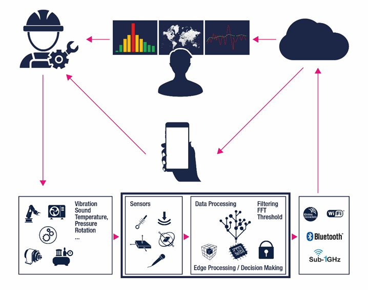
Figure 1 — Typical PM Application in Industry 4.0
To help identify small problems before they become big ones in expensive, sophisticated and potentially remote equipment, local decision making based on sensing data collected in (or near) the equipment forms the backbone of Industry 4.0. This requires sensor(s) with Edge Processing[13] and the ability to use Artificial Intelligence (AI) techniques as key technology in predictive maintenance application. With AI and edge processing directly in the sensor(s) or in the host controller such as FP-AI-MONITOR1[7] in STM32[8], data analysis and decision making can be done locally.
Figure 1 illustrates a typical predictive maintenance application. Here, the sensor(s) detects information from the equipment and passes the data to the host controller. In Industry 3.0, the raw sensor data describing the machine’s condition is streamed to operators directly, without any local processing or decision making. In Industry 4.0, the sensor data is processed locally by the host controller, where it can make decisions locally. The host controller allows the RF connectivity section to sleep, unless specific alert criteria requiring transmission is met. Human involvement only starts after receiving an alert message from the cloud. This approach reduces the data transferred to the cloud and reduces the power consumption of the local sensor node.
Going deeper, in implementing this sensing & decision-making block, there are four key steps in this approach: Significant Parameter Identification; Data Profiling; Sensor Selection, and the Decision Three Location Selection.
- Significant Parameter Identification
Many parameters can signal the health condition of a machine. Designers need to screen these significant parameter(s) based on their characteristics and their ability to predict the status of the machine. In the application scenario of Figure 2, parameters such as acoustics, temperature, and physical vibration in acceleration can each indicate the wear and tear on a heavy-duty bearing in a machine. Designers would study the parameters that could be used to predict a targeted 60% health condition of the bearing. The best scenario is when just one single parameter is sufficient in giving the most significant information and allowing the decision tree to judge 60% of the health condition it reaches.
In this example, the health condition of the machine is partitioned into four stages as listed in Table 1:
Table 1 — Machine Health Milestone
| Health Mark | Time Stamp | Machine condition | Action |
| 80% | t1 | Starting of Wear & Tear | Signal for repairing |
| 60% | t2 | Friction increase | Service required |
| 50% | t3 | Bearing start to crack | Replacement required |
| <30% | t4 | Urgent Replacement | Disaster |
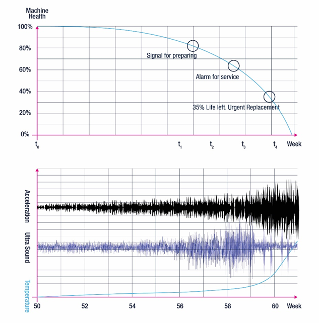
Figure 2 — Significant Parameter vs Machine Health
In specifying that an early warning be delivered when the heavy-duty bearing deteriorates to 60% of its health condition, Acceleration, Ultrasound, and Temperature vs Time (week) are captured and plotted in Figure 2 for the significant parameter study. From the graph, all three parameters can indicate the condition of the bearing. Some findings:
- Acceleration data gives a strong signal when the bearing runs into the breaking down stage after t3. However, it does not track the health condition of the bearing well before t3, which corresponds to 50% of the health of the machine. This means we can’t tell the machine’s health condition well before the bearing cracks. The singling from the accelerometer alone is not strong enough for early-stage wear & tear.
- Temperature data does not track the health condition of the bearing well until t4 when the bearing had already gone into the break-down stage. Whatever the cause, this disallows the temperature parameter from giving significant signal before the friction increase dramatically.
- The Ultrasound parameter effectively tracks bearing health condition and gives singling as early as t1. As friction increases, it gives a significant signal when the bearing is running into 60% mark of its health stage. From the data plotted however, the ultrasound signal started to lose track of the machine health condition when the bearing health dropped below 50% around t3. This is the result of the serious wear & tear and cracking that dramatically changed the bearing property and drives the vibration profile of the bearing out of the ultrasound range. In this stage, the strong vibration is being sensed by the accelerometer.
From this particular example, ultrasound is the significant parameter for predictive maintenance for 60% of the health warning.
- Data Profiling
Once the significant parameter is identified, the next step is to study the detailed data profile. Designers must evaluate different data processing functions and AI algorithms to provide a reliable prediction of the machine’s health.
Many data processing techniques are available for predictive maintenance applications. They can be summarized as using two main approaches: Time Domain and Frequency Domain[9]. Each has pros and cons.
- Using the time domain is simple, straightforward, and requires little processing power. The sensors’ output is always in the time domain. Root-Mean-Square (RMS), Average, or Peak detection on the time domain signal are the typical values to track. A decision flag can be obtained by threshold or amplitude comparison on the raw data or on processed data. The drawback to this approach is it only applies to simple waveform profiles. Some data profiles of real-world industrial applications are complicated, as they might combine vibrations from different mechanical parts along with ambient vibrations from other machines. Figure 3 illustrates an example data profile in the time domain.

Figure 3 — Example Acceleration Waveform in Time Domain
In this example, the vibration amplitude from the unbalancing is much larger than the vibration from it. So, this particular sensor arrangement, using RMS or Averaging or other signal processing technique under time domain, the data cannot effectively identify the vibration level from the output shaft.
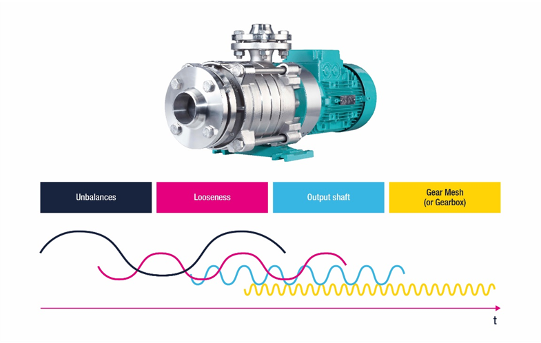
Figure 4 — Complex Waveform is the Sum of Multiple Waveforms
- There is a powerful signal processing tool for manage complicated signals, however. Figure 4 shows that this type of complex waveform is the sum of multiple simple waveforms. The Fast Fourier Transform (FFT) is an efficient tool for waveform profiling that converts the time domain data into the frequency domain and, from this vibrations from different parts are identified in the different frequency spectrum as Figure 5 illustrates.
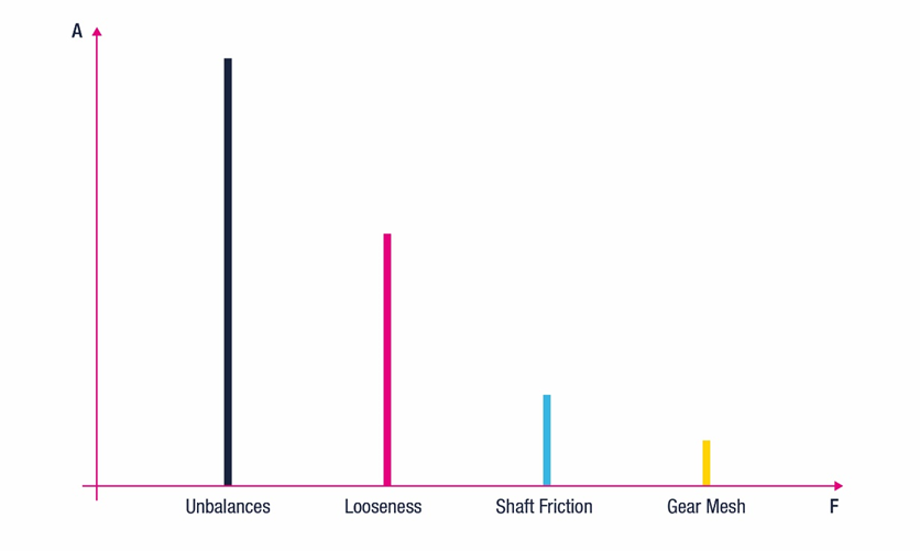
Figure 5 — Frequency Spectrum
The FFT separates vibration amplitudes of the different sources into different spectrum. Them, on top of the FFT, additional data processing techniques — Averaging, RMS, Peak, Neural Network, etc. — can be used for more data filtering and decision trees to achieve smarter decision making.
Parameter identification and data profiling requires some tools. There are some options:
- Professional measurement tools;
You can use professional off-the-shell measurement equipment to provide measurement data that is accurate and detailed. This equipment is highly recommended for demanding high-precision applications. .
- Evaluation or demo kits.
Sensor suppliers such as STMicroelectronics provide code-free evaluation kits (Figure 6). These small motherboards, like the STEVAL-MKI109V3, have sockets that accept the manufacturer’s sensors boards. Designers can choose the preferred sensor adaptor board and slot it into the motherboard. Some suppliers also offer a Graphical User Interface (GUI) to control the sensors. The GUI provides access to all of the sensor registers to configure and retrieve data without coding, and to provide useful arithmetic data processing functions. FFT is one of these functions (Figure 7).
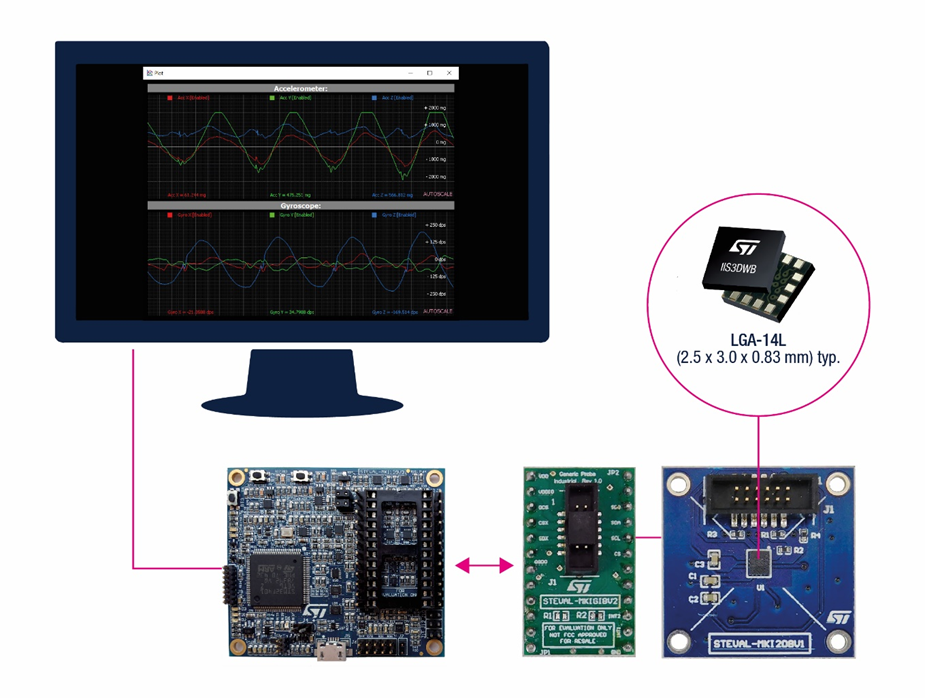
Figure 6 — Connection of STEVAL-MKI109V3 Based Evaluation Tool
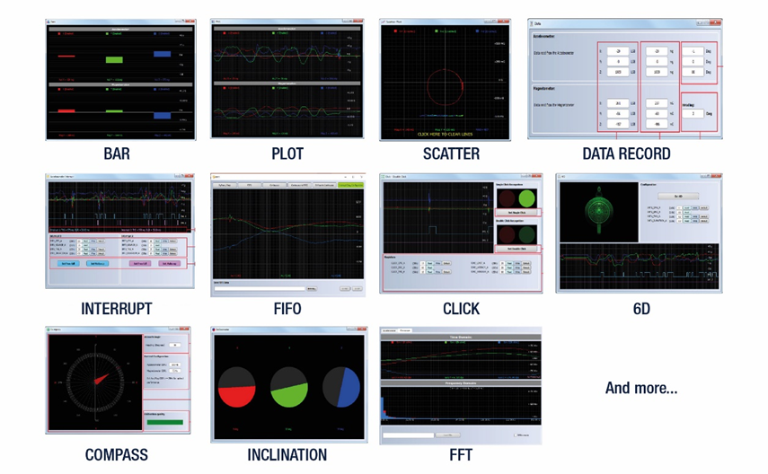
Figure 7 — Screenshots of STEVAL-MKI109V3 GUI
The code-free evaluation boards are recommended to assess the characteristics of the sensor and its suitability for the application. The boards can also perform initial data acquisition to start engineering algorithms and data analysis. Then, to move to prototypes or proofs of concept, suppliers may offer another powerful tool to greatly simplify and shorten the task: the STWIN development kit is an example:
- The STWIN wireless industrial node (STEVAL-STWINKT1B)[10][11] is a development kit and reference design that simplifies prototyping and testing of advanced industrial IoT applications such as condition monitoring and predictive maintenance.
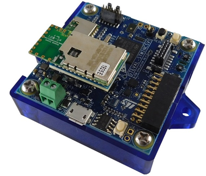
Figure 8 — STEVAL-STWINKT1B
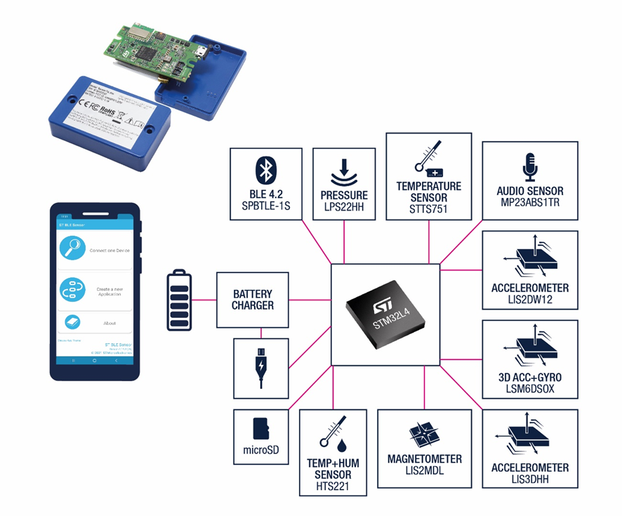
Figure 9 — SensorTile Box Works with Mobile Phone
Built around an ultra-low-power STM32 microcontroller and a wide range of industrial-grade sensors, including inertial sensors (vibration sensors, accelerometer, 6-axis IMU, magnetic sensors), environmental sensors (high accuracy temperature sensor, pressure sensor, humidity sensor), and high-performance microphones (both digital and analog, with ultrasound sensing capabilities), the kit supports exploration of all condition monitoring dimensions, especially the ones related to vibration analysis. The development kit is also complemented with a rich set of software packages and optimized firmware libraries, as well as a cloud dashboard application, to speed up design cycles for end-to-end solutions.
The kit supports Bluetooth® low energy wireless connectivity through an on-board module, and Wi-Fi connectivity through a special plugin expansion board (STEVAL-STWINWFV1). Wired connectivity is also supported via an on-board RS485 transceiver.
- Sensor Selection
With the data profile on hand, the next step is to select the appropriate sensor:
- Type of the sensor(s) based on the significant parameter(s) found in 1)
STMicroelectronics provides a full range of sensors from accelerometer, gyroscope, magnetometer, vibration sensor, microphone, pressure sensor, humidity sensor, temperature sensor, laser sensor, and infrared sensor, among others. Often industrial grade sensors assure higher performance and accuracy, better stability over temperature and time, and even assured production longevity.
- Range of the sensor, based on the measurement full scale and Sensitivity or significant frequency range (Bandwidth) found in 2)
Every sensor has its own maximum measurement range and frequency response bandwidth. Designers have to study these two parameters carefully to select the sensor that is best suited to their application. Figure 9 illustrates recommended part numbers for a range of predictive-maintenance application scenarios.
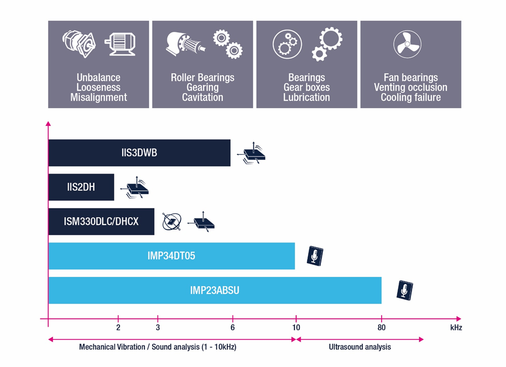
Figure 10 — Sensor Selection for Application Scenarios
- Decision Tree Location Selection
As a recognized leader in MEMS technology, STMicroelectronics is a pioneer in embedding edge-processing functions into its sensor products. A designer can partition the edge processing in the sensor or embed it in the host controller. The best choice depends on the complexity of the data processing and decision tree. The decision-making function within ST’s sensors are catalogued into three categories:
- Embedded Simple Logic
All of ST’s MEMS sensors feature embedded logic functions in the form of simple threshold comparisons. An Interrupt Flag is triggered once a preset amplitude and time-window threshold is met.
- Finite State Machine (FSM)[6]
A state machine is a mathematical abstraction used to design logic connections (Figure 10). The FSM is a behavioral model composed of a defined number of states and transitions between states, similar to a flow chart. The sensor can be configurated to generate a decision flag once the user-defined pattern is satisfied. Some ST sensors embed 16-state machines for decision making.
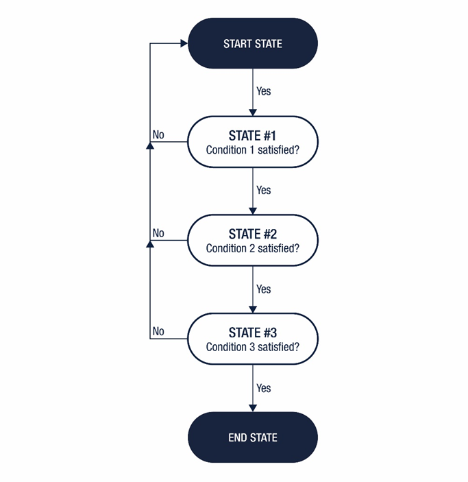
Figure 11 — Sensor Embedded Finite State Machine
- Machine Learning Core (MLC)[5]
An MLC is NOT made to process complicated data, so it can’t do an FFT. The MLC does allow some low-density algorithms that might otherwise run in the application processor to be moved to the MEMS sensor. This significantly reduces power consumption. An MLC can identify data patterns when they match a user-defined set of classes. The sensor can filter input data using a dedicated configurable computation block containing filters and features computed in a user-defined fixed time window. Machine learning processing is based on logical processing via a series of configurable nodes characterized by “if-then-else” conditions where the “feature” values are evaluated against defined thresholds (Figure 11).
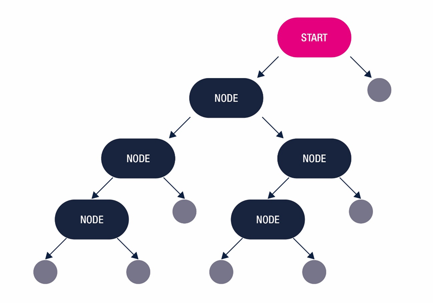
Figure 12 — Decision in MLC of a Sensor

Overall, as a fundamental part of Industry 4.0, sensors are essential components in predictive maintenance and, with inbuilt smart functions, can offload tasks from the host controller, making the entire system more efficient. As a MEMS sensor industry leader, ST provides a full range of sensors (accelerometers, gyroscopes, magnetometers, vibration sensors, microphones, pressure sensors, humidity sensors, temperature sensors, laser sensors, and infrared sensors, among others . For predictive maintenance and other applications, this wide range of products delivers a vital bridge between your innovative ideas and the actual application


